
AFPM Core Power Density Design
Estimate torque and iron-only kW/kg, compare assumptions, and export a design-review brief.
Core Power Density Sizer & RFQ Brief
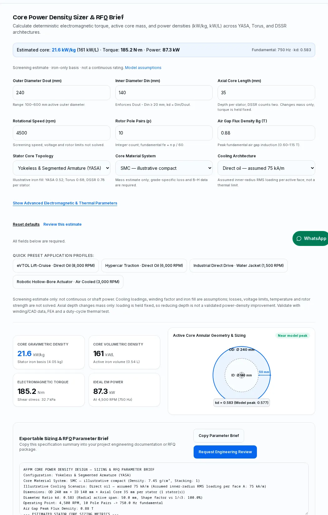
Calculate deterministic electromagnetic torque, active core mass, and power densities (kW/kg, kW/L) across YASA, Torus, and DSSR architectures.
Screening estimate · iron-only basis · not a continuous rating. Model assumptions
All fields below are required.
Screening estimate only: not continuous or shaft power. Cooling loadings, winding factor and iron fill are assumptions; losses, voltage limits, temperature and rotor strength are not solved. Axial depth changes mass only: loading is held fixed, so reducing depth is not a validated power-density improvement. Validate with winding/CAD data, FEA and a duty-cycle thermal test.
21.6 kW/kg
Stator iron basis (4.05 kg)
161 kW/L
Active iron volume (0.54 L)
185.2 N·m
Shear stress: 32.7 kPa
87.3 kW
At 4,500 RPM (750 Hz)
Exportable Sizing & RFQ Parameter Brief
Copy this specification summary into your project engineering documentation or RFQ package.
By AxialFluxCore · First recorded · Evidence reviewed .
Annual editorial review, with earlier corrections when simulation methodology, cooling benchmarks, or primary standards change. Public documents were checked on the review date; project-specific ratings require agreed validation methods and test evidence.
Evidence policy: linked manufacturer facts and publisher scopes are distinguished from editorial checklists. No grade-loss prediction without matched B-H data is asserted.
Four Core Principles of AFPM Power Density Sizing
Compare geometry before committing the design
Use the ideal torque and iron-mass estimates to prepare a validation brief. The tool does not calculate continuous or shaft output.
Traceable scope / standard: IEC 60034-2-3:2024 — Losses and efficiency of converter-fed AC motors
The diameter optimum is conditional
The selected torque shape factor peaks at kd = 1/√3. It is not a universal efficiency or installed power-density optimum.
Traceable scope / standard: Parviainen (2005): Design of Axial-Flux Permanent-Magnet Low-Speed Machines, §1.3.1, pp. 21–23
Cooling loadings are explicit assumptions
The 28 / 48 / 75 kA/m scenarios impose loading rather than solve temperature. Actual continuous duty needs a thermal test.
Traceable scope / standard: IEC 60034-1:2026 — Rating and performance
Compare equal mass and duty boundaries
DSSR counts both stators; all outputs exclude rotors, copper and housing. Full-motor density requires an actual BOM.
Basis: explicit model assumptions, arithmetic or engineering planning guidance; not measured machine performance.
Software capture, 2026-11-07: 240 mm OD, 140 mm ID, 35 mm depth per stator, YASA, illustrative SMC, direct-oil assumed loading of 75 kA/m per face, 4,500 rpm, 10 pole pairs and 0.88 T peak air-gap flux. The default result is 185.2 N·m, 87.3 kW ideal electromagnetic power and 21.6 kW/kg on the modeled iron-only basis. Reset defaults in the sizer to reproduce it. This is software evidence; it is not a physical test, customer case study or continuous motor rating.
1. Electromagnetic sizing and output boundaries
Use the sizer to compare geometry under stated assumptions, then validate the operating point.
This page uses radial conductors with inner-radius RMS linear loading A_in on each active face. The current sheet varies as A(r) = A_in·r_in/r. With aligned sinusoidal fields, mean shear is kw·Bg_peak·A(r)/√2. Integrating dT = 2π·shear·r²dr over each face gives T = π/(8√2)·kw·Bg·A_in·Dout³·kd(1−kd²)·N, using metres and A/m.
Power is T·2πn/60, before loss subtraction or voltage constraints. The assumed winding factor is 0.95, with two active faces. These inputs do not solve winding resistance, efficiency, back-EMF, saturation or temperature. A larger calculated output is an electromagnetic screening result; it cannot establish a shaft, continuous or certified rating.
Traceable scope / standard: Parviainen (2005): Design of Axial-Flux Permanent-Magnet Low-Speed Machines, §1.3.1, pp. 21–23
- 1. Define loading
- 2. Integrate torque
- 3. Validate duty
Planning basis: explicit calculator assumptions and engineering checks; not measured machine benchmarks.
| Quantity | Basis | Decision limit |
|---|---|---|
| Torque | Integrated radial current-sheet model | Requires actual winding harmonics and flux map |
| Power | Torque × mechanical speed | No losses or field weakening |
| Core density | Ideal power / modeled iron mass | Excludes copper, rotors and housing |
Traceable scope / standard: Parviainen (2005): Design of Axial-Flux Permanent-Magnet Low-Speed Machines, §1.3.1, pp. 21–23
2. Topology and the mass denominator
Count every stator before comparing core power density.
The model assumes iron occupancy of 0.52 for yokeless segmented teeth, 0.68 for a yoked Torus and 0.78 for each DSSR stator. These are illustrative fill fractions, not published topology averages. The same assumed face loading gives the same ideal torque at fixed diameters; changing topology changes the modeled mass, not a verified efficiency.
Axial length means depth per stator. DSSR has two stators, so both annular volumes are counted. The reported stator envelope is their sum; it excludes the rotor, magnets, air gaps and housing and is not installed motor volume. Reducing axial depth lowers the modeled mass while holding loading and torque fixed; this does not prove that the thinner core can accommodate the winding or carry flux. Replace fill factors with CAD volumes before selecting a topology or buying tooling.
Basis: explicit model assumptions, arithmetic or engineering planning guidance; not measured machine performance.
- 1. Count stators
- 2. Sum iron volume
- 3. Compare BOM
Planning basis: explicit calculator assumptions and engineering checks; not measured machine benchmarks.
| Topology | Stators / active faces | Illustrative iron fill |
|---|---|---|
| Yokeless segmented | 1 / 2 | 0.52 |
| Yoked Torus | 1 / 2 | 0.68 |
| DSSR | 2 / 2 | 0.78 per stator |
Basis: explicit model assumptions, arithmetic or engineering planning guidance; not measured machine performance.
3. Diameter ratio: a conditional optimum
The 0.577 maximum belongs to the chosen torque shape factor.
For fixed outer diameter, inner-radius loading and flux, f(k) = k(1−k²). Its derivative is 1−3k², giving k = 1/√3. The displayed score is f(k)/f(1/√3); it is a normalized torque factor, not an efficiency or a safety score.
The result changes if a different loading radius, constant shear, slot geometry or mass objective is held fixed. The tool accepts kd from 0.35 to 0.85 and a diameter difference of at least 20 mm as screening bounds. These bounds are not manufacturing approval. Check inner coil bends, bore clearance and tooth cross-section from the drawing.
Traceable scope / standard: Parviainen (2005): Design of Axial-Flux Permanent-Magnet Low-Speed Machines, §1.3.1, pp. 21–23
Computed curve, holding outer diameter, flux and inner-radius loading fixed. The peak is a model property; it is not measured motor efficiency.
- 1. Hold assumptions
- 2. Compare factor
- 3. Check slots
Planning basis: explicit calculator assumptions and engineering checks; not measured machine benchmarks.
| kd | Normalized shape factor | Interpretation |
|---|---|---|
| 0.4 | 87.3% | Computed at fixed outer diameter and A_in |
| 0.5 | 97.4% | Computed at fixed outer diameter and A_in |
| 0.5773502691896258 | 100.0% | Computed at fixed outer diameter and A_in |
| 0.7 | 92.8% | Computed at fixed outer diameter and A_in |
| 0.8 | 74.8% | Computed at fixed outer diameter and A_in |
Traceable scope / standard: Parviainen (2005): Design of Axial-Flux Permanent-Magnet Low-Speed Machines, §1.3.1, pp. 21–23
4. Materials: compare equal test conditions
The material selector changes a mass estimate; it does not predict material losses.
The sizer uses illustrative densities of 7.45 kg/L for SMC and 7.65 kg/L for NOES, with packing factors of 1.00 and 0.94. For amorphous ribbon it uses 7.18 kg/L and an assumed 0.85 stack factor. Obtain the actual compact density or finished stack volume before treating mass as a procurement input.
SMC supports three-dimensional component designs; steel and ribbon require attention to the lamination direction. No fixed frequency cutoff proves which material wins. Compare loss and B–H data at the same flux waveform, temperature, specimen geometry and processing state. Do not treat air-gap induction as tooth induction.
Traceable scope / standard: Höganäs — Somaloy coated powders for electromagnetic applications · Metglas Power Brochure — 2605SA1 typical properties, p. 9
- 1. Name grade
- 2. Match test data
- 3. Check core loss
Planning basis: explicit calculator assumptions and engineering checks; not measured machine benchmarks.
| Family | Mass assumption | Missing decision evidence |
|---|---|---|
| SMC | 7.45 kg/L; packing 1.00 | Named grade, compact density, B–H and loss map |
| NOES | 7.65 kg/L; packing 0.94 | Sheet thickness, stack and cut-edge losses |
| Amorphous | 7.18 kg/L; packing 0.85 | Anneal, stress and assembled-core loss |
Traceable scope / standard: Höganäs — Somaloy coated powders for electromagnetic applications · Metglas Power Brochure — 2605SA1 typical properties, p. 9
5. Thermal paths and hotspot uncertainty
Map the winding-to-coolant path before assigning a continuous rating.
The calculator contains no thermal network. Copper, slot liner, impregnation, tooth contact, cassette and coolant each introduce a thermal path. A compact with three-dimensional magnetic properties does not remove thermal contact resistance. Lamination orientation and interfaces must be represented in the thermal model.
Internal cooling channels are a candidate design route, not an automatic performance improvement. Removing iron changes flux density and strength while sealing adds manufacturing work. No verified project-specific percentage reduction in thermal resistance is available here; request a motorette experiment before crediting a gain.
Basis: explicit model assumptions, arithmetic or engineering planning guidance; not measured machine performance.
- 1. Map heat path
- 2. Measure contacts
- 3. Test hotspot
Planning basis: explicit calculator assumptions and engineering checks; not measured machine benchmarks.
| Thermal element | Required input | Verification |
|---|---|---|
| Winding to tooth | Contact and liner resistance | Motorette temperature mapping |
| Tooth to carrier | Assembly pressure and interface | Repeat after thermal cycling |
| Carrier to fluid | Flow, inlet temperature and wetted area | Pressure-drop and heat-balance test |
Basis: explicit model assumptions, arithmetic or engineering planning guidance; not measured machine performance.
6. Cooling choices are loading scenarios
Assumed 28 / 48 / 75 kA/m values enable comparison and do not certify heat extraction.
Selecting forced air, water jacket or direct oil assigns inner-radius RMS loading of 28, 48 or 75 kA/m per face. The resulting power ratio follows the imposed loading ratio. The model does not infer these loadings from coolant flow, winding area, ambient conditions or insulation temperature.
Natural convection must be assessed separately from forced air. A direct oil design also needs fluid/material compatibility, filtration, sealing and pump-loss checks. When thermal inputs are unknown, compare the scenarios and send the duty cycle for review; do not choose a continuous rating from the highest card.
Traceable scope / standard: IEC 60034-1:2026 — Rating and performance
- 1. Choose scenario
- 2. Specify coolant
- 3. Validate thermal
Planning basis: explicit calculator assumptions and engineering checks; not measured machine benchmarks.
| Scenario | Assumed A_in RMS per face | Still unknown |
|---|---|---|
| Forced air | 28 kA/m | Airflow, ambient and enclosure |
| Water jacket | 48 kA/m | Thermal interfaces, inlet and flow |
| Direct oil | 75 kA/m | Wetting, compatibility and pump power |
Traceable scope / standard: IEC 60034-1:2026 — Rating and performance
7. Slot fill and conductor loss
More copper area helps only after AC loss and assembly constraints are checked.
Do not compare a gross slot-fill percentage with a net copper fraction. Slot liners, enamel, turn clearance and impregnation consume space. A rectangular conductor can change manufacturability and resistance, while its AC loss depends on dimensions, frequency and local field.
The tool has no slot count, turns or wire size, so it cannot calculate current density or copper loss. Supply a winding drawing and measured resistance. Evaluate round wire, formed rectangular conductors and litz by assembled loss and cost rather than an unsupported universal fill-factor ranking.
Traceable scope / standard: IEC 60034-2-3:2024 — Losses and efficiency of converter-fed AC motors
- 1. Define net fill
- 2. Estimate AC loss
- 3. Trial winding
Planning basis: explicit calculator assumptions and engineering checks; not measured machine benchmarks.
| Option | Potential value | Cost or failure risk |
|---|---|---|
| Round wire | Flexible winding process | End turns and packing depend on process |
| Formed rectangular | Controlled geometry | Bend, enamel damage and AC proximity loss |
| Litz | High-frequency loss control | Termination labor and strand utilization |
Traceable scope / standard: IEC 60034-2-3:2024 — Losses and efficiency of converter-fed AC motors
8. Axial pull: local pressure is not net assembly load
Use a flux distribution and a structural load case, not a topology-wide force range.
For a locally normal field and negligible tangential field, magnetic pressure is approximately B²/(2μ0). A local 0.95 T field gives about 359 kPa. That arithmetic is not an average force over an annulus when 0.95 T is a sinusoidal peak. Spatial and time averaging and effective area must be specified.
Opposing faces can balance resultant force in an ideal symmetric assembly while each rotor disc still bends under attraction. Assembly, bearing offset and fault cases can break that balance. Retention material, fatigue allowables and gap deflection require structural analysis; this page provides no safe stress or force limit.
Basis: explicit model assumptions, arithmetic or engineering planning guidance; not measured machine performance.
- 1. Map pressure
- 2. Analyze discs
- 3. Check gap margin
Planning basis: explicit calculator assumptions and engineering checks; not measured machine benchmarks.
| Load case | Known calculation | Missing evidence |
|---|---|---|
| Local normal field | p ≈ B²/(2μ0) | Full normal/tangential flux map |
| Per-face attraction | Integrate pressure over area | Geometry, peak/average convention |
| Assembly imbalance | Difference of opposing face forces | Bearing compliance and tolerances |
Basis: explicit model assumptions, arithmetic or engineering planning guidance; not measured machine performance.
9. Inverter harmonics and voltage limits
Fundamental frequency alone cannot predict inverter-fed loss.
The tool calculates fe = n·p/60. It does not use carrier frequency, modulation, DC voltage, inductance or back-EMF. Raising speed at unchanged assumed torque therefore increases ideal power even when a real drive would enter field weakening or exceed its voltage limit.
IEC 60034-2-3:2024 describes converter-fed loss assessment within its scope; it is not a source for fixed SiC or GaN loss multipliers. Request loss maps with converter details and enough operating points to represent the intended duty. Agree treatment of motor, inverter and pump power.
Traceable scope / standard: IEC 60034-2-3:2024 — Losses and efficiency of converter-fed AC motors
- 1. Check voltage
- 2. Capture waveform
- 3. Measure loss
Planning basis: explicit calculator assumptions and engineering checks; not measured machine benchmarks.
| Input | Why it matters | Evidence needed |
|---|---|---|
| DC bus and back-EMF | Voltage feasibility at speed | Winding constants and drive map |
| PWM and current waveform | Additional core and copper losses | Waveforms and converter-fed test |
| Duty operating points | Time-weighted loss and heating | Torque-speed-duration schedule |
Traceable scope / standard: IEC 60034-2-3:2024 — Losses and efficiency of converter-fed AC motors
10. Air gap and tolerance allocation
A drawing-specific stack determines minimum running clearance.
The page cannot derive gap tolerance from outer diameter or power density. Start with a nominal gap and account for rotor runout, bearing motion, housing alignment, temperature and magnetic deflection. Static drawing clearance and minimum hot running clearance are different requirements.
Avoid a universal percentage torque penalty for a change in gap. Magnet thickness, leakage and saturation alter the sensitivity. Sweep the actual design in electromagnetic and structural models, then check assembly yield and scrap cost before tightening tolerances.
Basis: explicit model assumptions, arithmetic or engineering planning guidance; not measured machine performance.
- 1. Allocate stack
- 2. Sweep gap
- 3. Check yield
Planning basis: explicit calculator assumptions and engineering checks; not measured machine benchmarks.
| Contributor | Required definition | Minimum next step |
|---|---|---|
| Manufacturing | Datums, runout and flatness | Supplier capability review |
| Operating deflection | Speed, temperature and attraction | Coupled clearance analysis |
| Electromagnetic sensitivity | Actual magnet and tooth geometry | Gap sweep in FEA |
Basis: explicit model assumptions, arithmetic or engineering planning guidance; not measured machine performance.
11. Leakage and alternatives to extra iron
Check a three-dimensional flux path before assigning a gain to overhang or Halbach magnets.
Radial fringing, pole-to-pole leakage and local housing eddy currents depend on the complete magnetic circuit. Neither a fixed leakage percentage nor a universal casing clearance is supported by the inputs here. A conductive shield can introduce its own loss and must be evaluated in context.
Magnet overhang, changed pole pitch and Halbach arrangements are alternatives to compare, including magnet cost, assembly fixtures and retention. Use a common operating point and installed mass boundary; a reduction in one component can move cost or loss elsewhere.
Basis: explicit model assumptions, arithmetic or engineering planning guidance; not measured machine performance.
- 1. Model full field
- 2. Compare options
- 3. Include cost
Planning basis: explicit calculator assumptions and engineering checks; not measured machine benchmarks.
| Alternative | Potential benefit | Decision cost |
|---|---|---|
| Magnet overhang | Different edge flux capture | Magnet mass and retention |
| Halbach arrangement | Different field distribution | Magnetization and assembly complexity |
| Housing separation | Reduced stray-field coupling | Larger installed envelope |
Basis: explicit model assumptions, arithmetic or engineering planning guidance; not measured machine performance.
12. Core density versus complete motor density
Use a BOM for the full motor; no fixed mass multiplier is justified.
The tool divides ideal electromagnetic power by active iron mass. That denominator excludes windings, magnets, rotor discs, shaft, bearings, cassette, cooling hardware and housing. Its kW/kg result cannot be compared directly with a complete motor benchmark.
As a hypothetical arithmetic example, 150 kW divided by 5 kg iron is 30 kW/kg on a core basis. If the complete assembly is 25 kg, the same assumed power is 6 kW/kg. These are illustrative denominators, not tested continuous or peak ratings. Define whether inverter, coolant and pump are included.
Basis: explicit model assumptions, arithmetic or engineering planning guidance; not measured machine performance.
- 1. Define boundary
- 2. Sum full BOM
- 3. Compare like duty
Planning basis: explicit calculator assumptions and engineering checks; not measured machine benchmarks.
| Boundary | Hypothetical mass at 150 kW | Arithmetic density |
|---|---|---|
| Iron only | 5 kg | 30 kW/kg |
| Complete dry motor | 25 kg | 6 kW/kg |
| Installed system | Unknown: add drive and cooling | N/A until system BOM exists |
Basis: explicit model assumptions, arithmetic or engineering planning guidance; not measured machine performance.
13. Speed, pole pairs and loss-map coverage
Compute frequency exactly, then check the material and drive at that point.
For the default point, 4,500 rpm with 10 pole pairs produces 750 Hz. An 8,000 rpm point with 8 pole pairs produces approximately 1,067 Hz. These are arithmetic identities, not application recommendations or evidence of a safe rotor speed.
At higher frequency, request material data at the relevant flux waveform and temperature. At higher speed, check centrifugal retention, bearings and rotor dynamics. Reducing pole count changes winding and magnetic geometry; it is not a free remedy for core loss.
Basis: explicit model assumptions, arithmetic or engineering planning guidance; not measured machine performance.
- 1. Calculate fe
- 2. Check loss map
- 3. Check rotor
Planning basis: explicit calculator assumptions and engineering checks; not measured machine benchmarks.
| Illustrative point | Pole pairs | Computed fundamental |
|---|---|---|
| 4,500 rpm | 10 | 750 Hz |
| 8,000 rpm | 8 | 1,066.7 Hz |
| 1,500 rpm | 16 | 400 Hz |
Basis: explicit model assumptions, arithmetic or engineering planning guidance; not measured machine performance.
14. Manufacturing and quality evidence
Replace generic material promises with lot and component acceptance data.
For pressed SMC, specify powder grade, compaction route, density, heat treatment and coating compatibility. For laminations, specify sheet grade, orientation, cutting, burr control and joining. For ribbon, identify anneal, packing and handling conditions. Each route affects the assembled component.
Set dimensional, magnetic and mechanical acceptance criteria from the actual drawing and load case. A material coupon test does not prove finished-tooth retention strength or assembly reliability. Do not use a coating-thickness method as proof of insulation on individual buried powder particles.
Traceable scope / standard: Höganäs — Somaloy coated powders for electromagnetic applications
- 1. Specify process
- 2. Approve samples
- 3. Control lots
Planning basis: explicit calculator assumptions and engineering checks; not measured machine benchmarks.
| Route | Request from supplier | Production risk |
|---|---|---|
| SMC | Lot traceability and finished-compact data | Tooling, density gradient and brittle handling |
| NOES | Cut-edge and joined-stack data | Burrs, shorts and assembly labor |
| Ribbon | Anneal and handling record | Packing, damage and mounting stress |
Traceable scope / standard: Höganäs — Somaloy coated powders for electromagnetic applications
15. Choose by duty, cost and scenario fit
A maximum screening density is one objective among several.
Engineering and procurement should compare the same shaft duty, installed mass, coolant conditions and reliability requirement. Tooling cost, annual volume, scrap, winding labor and cooling auxiliaries can outweigh an apparent core-mass advantage.
Keep at least one simpler alternative in the comparison: a yoked stator, a different loading target or a larger envelope. If a route needs unproven sealing or tight clearances, request a prototype milestone and costed acceptance plan before volume tooling.
Basis: explicit model assumptions, arithmetic or engineering planning guidance; not measured machine performance.
- 1. Agree objectives
- 2. Compare tradeoffs
- 3. Stage prototype
Planning basis: explicit calculator assumptions and engineering checks; not measured machine benchmarks.
| Priority | Candidate comparison | Gate before selection |
|---|---|---|
| Lowest iron mass | Yokeless versus yoked CAD | Retention and full BOM |
| Continuous duty | Air versus indirect/direct liquid | Thermal test and auxiliary power |
| Volume production | Pressed versus cut/assembled core | Costed yield and tooling plan |
Basis: explicit model assumptions, arithmetic or engineering planning guidance; not measured machine performance.
16. RFQ handoff and minimum validation package
Export the assumptions and evidence gaps along with the numbers.
The parameter brief carries geometry, operating point, both density denominators, assumed loading and boundary warnings. It is a screening request, not a released motor specification. Invalid inputs suppress the result; reset defaults or send the available drawing and duty requirements for review.
For an actionable RFQ, add torque-speed-duration data, winding details, installed mass boundary, inlet temperature and flow, voltage and inverter waveform, rotor clearance requirements, annual volume and sample acceptance criteria. Ask the supplier to identify what is measured, modeled and still unknown.
Traceable scope / standard: IEC 60034-2-3:2024 — Losses and efficiency of converter-fed AC motors
- 1. Export assumptions
- 2. Attach evidence
- 3. Request review
Planning basis: explicit calculator assumptions and engineering checks; not measured machine benchmarks.
| Package | Minimum supplied information | Next action |
|---|---|---|
| Electromagnetic | Geometry, poles, winding, voltage and duty | Check torque, loss and drive feasibility |
| Thermal/mechanical | Coolant boundary and minimum gap | Plan hotspot and retention validation |
| Procurement | Volume, drawing revision and acceptance | Quote samples, tooling and production separately |
Traceable scope / standard: IEC 60034-2-3:2024 — Losses and efficiency of converter-fed AC motors
Hypothetical inputs and next decisions
Computed preset examples across aerospace, automotive and robotics. Each uses the same screening assumptions and identifies the next validation step.
eVTOL Lift-Cruise · Direct Oil (8,000 RPM)
Application Context: Hypothetical 200 mm OD × 115 mm ID × 28 mm per-stator depth; 8000 rpm.
Initial Bottleneck: Compare an operating point without confusing core-only density with a motor rating.
Engineering Execution: Apply the named preset using the same assumed loading, fill fraction and sinusoidal model as the sizer.
Outcome: Calculated only: 103.6 N·m, 86.8 kW ideal power, 2.28 kg iron, 38.0 kW/kg iron. Next: check voltage, loss map, hotspot and retention.
Illustrative model output; no measured or continuous performance claim. Select the matching preset above to reproduce it.
Hypercar Traction · Direct Oil (6,000 RPM)
Application Context: Hypothetical 260 mm OD × 150 mm ID × 40 mm per-stator depth; 6000 rpm.
Initial Bottleneck: Compare an operating point without confusing core-only density with a motor rating.
Engineering Execution: Apply the named preset using the same assumed loading, fill fraction and sinusoidal model as the sizer.
Outcome: Calculated only: 246.3 N·m, 154.7 kW ideal power, 5.30 kg iron, 29.2 kW/kg iron. Next: check voltage, loss map, hotspot and retention.
Illustrative model output; no measured or continuous performance claim. Select the matching preset above to reproduce it.
Robotic Hollow-Bore Actuator · Air Cooled (3,000 RPM)
Application Context: Hypothetical 140 mm OD × 90 mm ID × 22 mm per-stator depth; 3000 rpm.
Initial Bottleneck: Compare an operating point without confusing core-only density with a motor rating.
Engineering Execution: Apply the named preset using the same assumed loading, fill fraction and sinusoidal model as the sizer.
Outcome: Calculated only: 11.9 N·m, 3.7 kW ideal power, 0.77 kg iron, 4.9 kW/kg iron. Next: check voltage, loss map, hotspot and retention.
Illustrative model output; no measured or continuous performance claim. Select the matching preset above to reproduce it.
Frequently Asked Questions (FAQ)
In-depth engineering answers covering sizing equations, core materials, thermal extraction, and manufacturing tolerances.
Sizing & Results
Is this a continuous power calculator?
No. It calculates ideal electromagnetic power under assumed loading. Continuous output needs losses, coolant conditions and a thermal duty test.
Why distinguish RMS current loading from peak flux density?
Their sinusoidal averages differ. The model combines peak flux density with RMS inner-radius current loading using the 1/√2 factor and integrates each active face once.
Where is current loading defined?
At the inner radius of each active face. The RMS current sheet is assumed to fall with radius as A_in·r_in/r; it is not slot current density in A/mm².
Does kd = 0.577 maximize every motor?
No. It maximizes the selected k(1−k²) shape factor at fixed outer diameter, inner-radius loading and flux. Packaging and other objectives can shift the choice.
What does the shape-factor score mean?
It is the torque shape factor relative to its mathematical maximum, expressed as a percentage. It is not efficiency or design approval.
How do I recover from an empty or invalid input?
Correct the highlighted field or use Reset defaults. Results and export are withheld until every required input passes validation; contact is still available.
Materials & Topology
Does selecting SMC prove lower core loss?
No. Material selection changes illustrative mass parameters. Request grade-specific loss and B–H data under representative conditions.
Why is DSSR heavier in this model?
It counts two stators at the entered depth per stator. The fixed iron fractions are assumptions; replace them with CAD volumes for an actual topology comparison.
Does YASA always save half the iron mass?
No universal percentage is claimed. Yoke removal changes the flux path and structure; quantify the difference using a common duty and full component geometry.
Is 2605SA1 a nanocrystalline material?
It is treated here as Fe-based amorphous ribbon. Do not interchange its grade data with nanocrystalline alloys.
Are the density and stacking values guaranteed?
No. They are mass-screening inputs. Confirm the actual compact density, packing, processing and drawing revision with the supplier.
Can I use air-gap flux as tooth flux?
No. Tooth cross-section, slot opening, leakage and saturation alter local induction. A magnetic circuit or FEA is needed.
Thermal & Drive
Do the cooling scenarios set safe current limits?
No. The 28, 48 and 75 kA/m loadings are imposed assumptions. The tool has no thermal solver or universal current-density limit.
Is natural convection equivalent to forced air?
No. The air scenario means forced air. Natural convection needs its own boundary conditions and heat-transfer evaluation.
Does power always grow linearly with speed?
Only in the calculation at constant assumed torque. Real voltage, loss, field-weakening and rotor limits can prevent that operating point.
How is electrical frequency calculated?
Multiply rpm by pole pairs and divide by 60. For 4,500 rpm and 10 pole pairs the fundamental is 750 Hz; PWM harmonics are additional.
What is missing for a continuous rating?
Copper and core losses, thermal contacts, coolant inlet and flow, ambient, duty duration, temperature limits and measured hotspot behavior.
Does IEC 60034-1 establish a universal kW/kg limit?
No. The 2026 edition is a rating framework within its scope, excluding rail and road vehicle machines. Agree the standards applicable to the project.
Validation & Procurement
Can I compare this kW/kg with a complete motor benchmark?
Only after matching mass boundary, power definition, duty duration and cooling. The tool denominator contains iron only.
Is the envelope output installed motor kW/L?
No. It uses the sum of stator annular envelopes, excluding rotors, magnets, air gaps and housing.
Does 359 kPa determine the total axial force?
No. It is approximate local pressure at a normal field of 0.95 T. Integrate the actual pressure distribution and distinguish local peak from average.
What if clipboard access is denied?
Use the labeled read-only parameter brief and select its text manually. The same brief is included in the engineering-review contact link.
Do the example scenarios represent customer results?
No. They are computed from the labeled presets with the same screening model. They describe the next validation decision, not tested outcomes.
What should accompany the parameter brief?
Attach the drawing, torque-speed-duration duty, winding and inverter data, coolant boundaries, mass definition, volume and acceptance criteria.
Primary Standards & Traceable References
Checked on 2026-11-07. Catalogue scopes and primary-source sections are linked below. Calculator assumptions are editorial screening choices; sources do not certify this tool or its outputs. Application-specific compliance must be agreed separately.
Parviainen (2005): Design of Axial-Flux Permanent-Magnet Low-Speed Machines, §1.3.1, pp. 21–23
Primary doctoral research: radial current-loading distribution and the ideal diameter-ratio shape factor. The calculator adapts the ideal model to aligned sinusoidal excitation; it does not reproduce a measured motor.
IEC 60034-1:2026 — Rating and performance
Edition 15, published 2026-03-13, replaces 2022. Rating framework within its scope; rail and road vehicle machines are excluded. Agree application-specific requirements; no topology-specific kW/kg limit follows from this catalogue scope.
IEC 60034-2-3:2024 — Losses and efficiency of converter-fed AC motors
Edition 2, published 2024-03-12. Describes testing and loss interpolation across operating points, including field weakening. It supplies no universal PWM loss multiplier or continuous current-loading limit.
Metglas Power Brochure — 2605SA1 typical properties, p. 9
Manufacturer transformer-material brochure: typical density 7.18 g/cm³ and saturation induction 1.56 T; values are not guaranteed. Transformer loss curves do not establish motor loss under rotating flux or PWM.
Höganäs — Somaloy coated powders for electromagnetic applications
Manufacturer guidance on soft magnetic composites and three-dimensional component design. Grade, pressing and heat treatment must be specified; this is not evidence for a universal loss or strength threshold.
Request an AFPM Core Power Density Design Review
Send your preliminary envelope dimensions, rotational speed targets, cooling conditions, and annual quantity requirements. Use the inquiry to agree on the scope of an electromagnetic and manufacturing review before committing to prototype tooling.
Direct inquiry contact: [email protected]