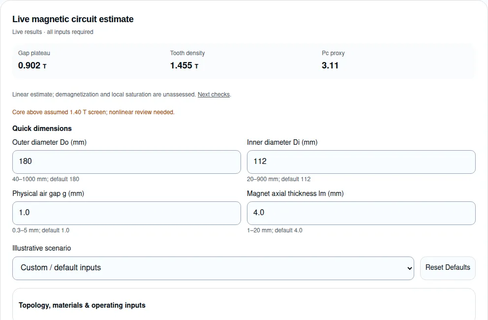
Linear estimate; demagnetization and local saturation are unassessed. Next checks.
Core above assumed 1.40 T screen; nonlinear review needed.
Core screen: above screen (assumed 1.40 T level)
Demagnetization is unassessed. Obtain temperature-specific magnet B–H/J–H curves and check peak opposing current and fault conditions.
Core density is near or above the assumed screening level. The fixed-permeability estimate may overstate flux; increase core area or run nonlinear FEA.
Model assumptions & detailed results
Ag = Am; At = 0.62 Ag; Ay = 0.65 At; fixed μr; μrec = 1.05. Effective series path: 2.30 mm total gap and 8.00 mm total magnet length, with one equivalent tooth. Two equal yoke branches are assumed where a stator return yoke is present. Rotor back-iron is omitted; topology comparisons do not establish an optimum.
Electrical frequency (not PWM)
400.0 Hz
Flux per pole
0.633 mWb
Pole area
701.8 mm²
Rgap (total external gap)
2.608 MA/Wb
Rtooth
0.114 MA/Wb
Ryoke (equivalent parallel pair)
N/A — no stator return yoke
Yoke density
N/A — through-flux approximation
Gap fundamental amplitude
1.039 T
Br(T), linear reference
1.220 T
The fundamental amplitude assumes a rectangular pole waveform and can exceed its plateau value. Leakage is a heuristic external-reluctance penalty. Read the equations and limitations.
Rgap = 2.608, Rtooth = 0.114, Ry,eq = N/A MA/Wb. Magnet internal reluctance affects the flux estimate but is excluded from the external reluctance shares. See all assumptions.
Four decisions the estimate can support
Confirm the flux path before selecting a core. YASA omits the stator yoke; rotor paths remain part of the real machine. Do not transfer the simplified circuit unchanged between architectures. [S1]
Use material data at its stated conditions. A maximum permeability is not the operating permeability, and B at a specified H is not a saturation limit. [S2]
Request comparable loss evidence. Check specimen type, waveform and frequency before comparing ring and electrical-steel measurements. [S3][S4]
Leave magnet safety open until hot curves and current are known. A geometry proxy alone cannot establish a demagnetization margin. [S5][S6]
Method: a declared effective flux tube
The following equations describe this implementation, not a validated complete-machine solver. Use SI units internally: lengths in m, areas in m², reluctance in A/Wb; displayed MA/Wb is 10⁶ A/Wb. μ0 = 4π × 10⁻⁷ H/m.
Ag = Am = π(Do² − Di²) αp / (8p); At = 0.62 Ag; Ay = 0.65 At
g_eff = kc g; Rg = gΣ/(μ0 Ag); Rt = lt/(μ0 μr At)
ly = π Rmean / p; Ry,eq = ly/(2 μ0 μr Ay), or 0 without a stator return yoke
Here gΣ and lmΣ are the effective total gap and magnet lengths in the selected approximation. kσ is a heuristic penalty on external reluctance, not an explicit leakage branch. The geometry-only Pc proxy excludes core reluctance and is not the actual magnet B/(μ0|H|) load-line coefficient. Ccore describes linear core reluctance; it is not a nonlinear saturation factor. The source term uses remanence and recoil permeability, not intrinsic coercivity Hcj.
Model assumptions and what to replace before design release
Quantity
Current assumption
Required engineering evidence
Tooth / yoke area
At = 0.62 Ag; Ay = 0.65 At
Net CAD areas and local tooth-root geometry
Core
One equivalent tooth; constant μr
Actual path lengths, parallel branches and nonlinear B–H data
Return yoke
Two equal half-flux branches; Ry,eq is half the single-branch reluctance
Topology-specific return circuit and rotor back-iron
Gap field
Uniform radial field; rectangular pole waveform
Radial slices and 3D fringing/leakage analysis
Magnet
Am = Ag; constant μrec = 1.05; linear reversible Br(T)
Supplier curves at temperature, current reaction and local field
Check radial variation before trusting a mean-radius correction
Radial slotting check. Slot pitch τs(r) = 2πr/Qs changes with radius. Slot-opening width may also vary; the direction and size of the local Carter correction require actual geometry. Compare radial slices rather than assuming a universal percentage gradient.
The calculator accepts kc as an input; it does not derive it from a slot sketch. Record slot count Qs, slot opening bs(r), tooth profile and minimum operating gap. Compare inner, mean and outer slices, then refine where gradients are large. This is an engineering check recommendation, not a fixed validated number of slices or a predicted gain.
Material evidence: preserve the grade and test conditions
Höganäs lists the following typical portfolio data at 800 MPa compaction and 1 T, 5 × 5 mm cross-section. These measured examples do not calibrate the calculator’s illustrative candidates. [S2]
Published Somaloy data — 2025 portfolio p. 4; not complete-machine predictions
Grade
Density (g/cm³)
B at 10,000 A/m (T)
Maximum μr
400 Hz loss (W/kg)
1 kHz loss (W/kg)
Somaloy 700 3P
7.57
1.61
850
45
132
Somaloy 1000 3P
7.56
1.63
950
46
143
The supplier warns that ring-component data and sheet test data are not directly comparable. Confirm density, heat treatment and section size, then compare under a common component duty. Electrical steel also needs an orientation and stacking specification; the calculator omits those effects. [S2][S4]
Loss and efficiency: known inputs, missing outputs
Material loss comparison workflow. Separate electrical fundamental frequency from PWM harmonics. Include both in the excitation specification; a geometry-only magnetic circuit cannot establish a universal SMC-versus-steel crossover frequency or efficiency gain.
What this tool establishes and what remains unknown
Decision item
Known from this page
Unknown / next evidence
Fundamental frequency
f_e = p n/60
PWM harmonic amplitudes and local B(t)
Material loss
Published specimen values at stated conditions
Actual part loss map, temperature and rotational flux
SMC versus steel
Different specimen methods and processing conditions
Matched component tests; no universal crossover is established
Efficiency / cooling
Not calculated
Copper, magnet, mechanical and inverter losses; thermal network
IEC measurement scopes help specify evidence, not predict machine efficiency. Keep the fundamental and carrier excitation separate and ask the laboratory to document the waveform and specimen preparation. [S3][S4]
Topology scope: use the model for sensitivities within a concept
Effective path counts used by this implementation — approximations, not full machine circuits
Concept
Gap / magnet count
Stator return yoke
Boundary
YASA / TORUS-NS
2 / 2
Omitted
One equivalent through-flux tooth; rotor return paths omitted
TORUS-NN
2 / 2
Equivalent pair included
Parallel paths are collapsed; needs a topology-specific branch network
SSSR
1 / 1
Equivalent pair included
One gap face; unbalanced axial attraction is not calculated
AFIR
2 / 1
Equivalent pair included
Effective surrogate; two stators and actual magnet arrangement need separate modeling
The original YASA paper supports the absence of its stator yoke. Other path counts above are implementation assumptions; they do not prove torque, mass, efficiency or temperature superiority. [S1]
Axial force validation. For a gap-dominated field, pressure scales approximately as B²/(2μ0). A symmetric nominal layout does not establish bearing stability. Evaluate the net restoring force with a stated displacement sign convention, structural compliance and the full tolerance stack. No force or stiffness value is predicted by this tool.
Risks, cost trade-offs and practical alternatives
Decision risks and the smallest useful follow-up
Risk
Consequence
Mitigation / alternative
Mistaking a proxy for safety approval
Demagnetization or an unsuitable core can remain undetected
Request hot curves and peak-current analysis; leave release status open
Unmodeled local saturation or leakage
Linear flux estimate can be overstated
Use net CAD sections and nonlinear radial/3D analysis
Choosing a material from unmatched loss data
Cooling and efficiency targets may be missed
Compare a common component geometry and waveform; test both candidates
Committing tooling before process qualification
Tooling iterations, scrap and sample delays
Request density and dimensional capability evidence; compare a low-volume sample route
Symmetry assumed across real tolerances
Rotor contact, bearing load or gap closure
Couple force-displacement and structural checks with thermal growth
Demagnetization remains a separate engineering decision
Evidence needed for a demagnetization decision. No numerical knee or safe Pc threshold is inferred here. Use supplier curves at the worst magnet temperature and evaluate armature reaction and fault conditions; see source S5.
The default N45SH reference uses typical Br20 = 1.35 T and αBr = −0.12%/°C from Arnold’s sheet. Its coefficient note covers 20–150°C; higher calculator temperatures are visibly marked as extrapolation. Other magnet rows are illustrative inputs. None of these choices supplies a temperature-dependent intrinsic knee or a safe operating temperature rating. [S5]
Request the actual grade’s B–H and J–H curves at the hottest local magnet temperature, then evaluate the most adverse opposing current and fault case. Geometry affects an operating slope, but safety requires the full magnetic circuit and local field distribution. [S5][S6]
Worked input scenarios — calculated examples, not customer cases
These are the same four presets offered in the tool. Values are calculated by this page’s model with the declared assumptions; no prototype tests, torque gains or production outcomes are claimed. Load a preset to inspect every input or export the summary.
Reproducible model examples — no-load estimates, reviewed 2026-10-25
Scenario
Do / Di (mm)
g / lm (mm)
p / rpm
Gap / tooth (T)
Pc proxy
Next action
eVTOL / Aerospace High-Speed YASA
180 / 112
1.0 / 4.0
8 / 4500
0.902 / 1.454
3.11
Inspect assumptions, obtain actual curves and request engineering review
EV Direct-Drive Traction TORUS-NS
240 / 150
1.2 / 5.0
10 / 3000
0.870 / 1.403
3.15
Inspect assumptions, obtain actual curves and request engineering review
Robotic Joint Compact Actuator SSSR
160 / 105
0.8 / 3.5
14 / 1200
0.963 / 1.553
3.55
Inspect assumptions, obtain actual curves and request engineering review
Marine Pod Propulsion AFIR
350 / 220
1.5 / 6.0
16 / 1500
0.688 / 1.110
1.47
Inspect assumptions, obtain actual curves and request engineering review
Original software execution captured 2026-10-25, with default inputs and results shown above the detailed model controls. Reproduce it with Reset Defaults and View Text Export. The crop excludes site navigation and floating contact controls. This is evidence of calculator execution; it is not a magnet test, prototype measurement or customer endorsement.
First version 2026-10-25 · Technical review 2026-10-25. The first-version date records creation, not a verified public publication date.
Review policy: AxialFluxCore will recheck the source editions, material conditions and model assumptions within six months of this review, or sooner when a cited datasheet or the model changes. Send corrections through the engineering inquiry form.
Public source scope checked 2026-10-25. Model equations, screening levels and topology surrogates are this page’s declared assumptions; citations do not imply third-party validation of the tool. Public evidence is insufficient to claim universal loss savings, magnet safety thresholds, certification or delivery time.
[S1] · 2007 · IEEE IEMDC · DOI 10.1109/IEMDC.2007.382753
Grade/process-specific ring-sample properties. Maximum permeability and induction at a specified field are not a constant permeability or a saturation knee.
[S3] · 2018 · amendment 1 published 2021; public scope checked 2026-10-25
Soft metallic and powder materials, excluding electrical steels and soft ferrites; 20 Hz–100 kHz. This page uses the public scope, not the paid test procedure.
[S4] · 2016 · 2018 corrigendum; public scope checked 2026-10-25
Grain-oriented and non-oriented strip/sheet; Epstein-frame AC measurements at 400 Hz–10 kHz. A test method does not prescribe a material loss coefficient.
Typical Br and reversible coefficient plus temperature-dependent B–H/J–H curves. Actual properties vary with magnet size and shape; no universal safe Pc is specified here.
Explains Pc as an operating slope and the assumptions behind open-circuit approximations. It does not validate this simplified motor model.
Frequently asked engineering questions
Using and interpreting the estimate
What does the AFPM core magnetic circuit design tool calculate?
It estimates no-load gap flux, equivalent tooth/yoke density, external reluctances, electrical frequency and a geometry-only Pc proxy. It uses constant material permeability and simplified topology counts, so the results support sensitivity analysis rather than design release.
Which inputs should I change first?
Start with outer/inner diameter, physical gap and magnet thickness. Then open topology, materials and operating inputs. All fields are required; defaults and allowed ranges appear beside each numerical field.
Does a higher Pc proxy mean my magnets are safe?
No. This proxy excludes core reluctance, local fields and armature reaction. Hot B–H/J–H curves, peak opposing current and fault conditions are needed to assess irreversible demagnetization; no safety margin is calculated.
Why can the fundamental amplitude exceed the gap plateau?
For an ideal rectangular pole waveform, the first spatial Fourier amplitude is (4/π) Bg sin(παp/2). That amplitude can exceed the local plateau. Real field shape, slotting and radial variation require field analysis.
How do I recover from a blank or invalid input?
Correct the marked field using decimal digits and a dot within its displayed range, or use Reset Defaults. Invalid combinations suppress the result and export. If dimensions are unavailable, send a drawing through the engineering inquiry form.
How do I export my input and result?
Use Copy MEC Sizing Summary or View Text Export. If clipboard access fails, a status message appears and the selectable export opens automatically. The summary includes every numerical input and the model limitations.
Materials and model boundaries
Are the core candidates qualified material grades?
No. They are illustrative constant-permeability candidates with explicitly assumed screening levels. Obtain the selected supplier grade, density, heat treatment, B–H curve and loss map before applying the estimate to a component.
Does the tool solve magnetic saturation?
No. It compares modeled core density with an assumed screening level while keeping permeability constant. Near or above the screen, flux may be overstated; use a nonlinear model with actual B–H data.
Is SMC always lower loss than thin electrical steel?
No universal crossover frequency is established here. Compare matched flux waveforms, temperature, frequency, component cross-section and manufacturing condition. Ring-sample and Epstein-frame results require careful normalization before a component decision.
Is the electrical frequency the PWM carrier frequency?
No. The electrical fundamental is pole pairs × rpm / 60. PWM carrier harmonics add a different excitation spectrum; this tool calculates neither harmonic losses nor efficiency.
Which magnetic test method applies?
IEC 60404-6 covers AC ring measurements for the soft materials in its scope, excluding electrical steels and soft ferrites. IEC 60404-10 covers electrical steel at 400 Hz–10 kHz. Confirm the applicable edition, specimen geometry and excitation with the test laboratory.
Topology and engineering handoff
Why is stator return-yoke reluctance absent in the YASA approximation?
The YASA stator has separate tooth segments without a stator yoke. This model omits stator return-yoke reluctance for YASA and its TORUS-NS through-flux approximation. Rotor return paths still exist and are omitted from this simplified estimate.
Can I rank YASA, TORUS and AFIR efficiency with these outputs?
No. Their actual branch circuits, rotor back-iron, tooth areas, winding currents and cooling differ. The topology counts are declared approximations; use architecture-specific electromagnetic and thermal models for comparisons.
Why check inner and outer radius separately?
Slot pitch changes with radius, and the slot opening may change too. A mean-radius correction does not bound local field crowding. Use the actual slot profile and compare radial slices; no universal Carter gradient is assumed.
Does a symmetric dual-rotor layout remove bearing risk?
No. Nominal axial-force balance does not establish stability under runout, thermal growth, disc deflection or bearing compliance. Evaluate force versus displacement and the mechanical tolerance stack.
What should an engineering inquiry include?
Attach the exported summary, topology sketch, tooth and yoke CAD, minimum/nominal/maximum gaps, material B–H and loss curves, magnet thermal curves, speed/current duty, cooling and intended sample quantity. Request a review of the missing evidence before tooling release.
Advance Your AFPM Core from 1D MEC to 3D FEA & Prototyping
Send the exported input summary, topology sketch, tooth/yoke CAD, gap tolerance stack, material curves and current/temperature duty. Identify the missing evidence before choosing a prototype or tooling route.